Can an experiment help in debates about decision theory?

Every philosophical decision theorist has an opinion on Newcomb’s puzzle. I won’t explain it here – if you don’t know what it is, try this.

Instead, consider a much more ordinary gamble:

You have two options. Option A and Option B. Here are the possible outcomes of each.

Option A: with probability $\frac{1}{3}$, you get nothing, with probability $\frac{2}{3}$ you get $40.

Option B: with probability $\frac{2}{3}$ you get $10, and with probability $\frac{1}{3}$ you get $50.

Some people will prefer the option A, which runs a risk of getting nothing, but brings a bigger chance at a large prize. Others will prefer the lower risk option B. Either choice can be rational, depending on your attitude to money and risk.[1]

We can now modify this gamble to resemble a Newcomb case. We would need to add a backstory to explain how the probabilities are determined. Here’s one.

We’ve looked at the genetics of people offered these types of gambles, and we can use that information to predict how people will choose. Our information is not great, but it usually lets us predict people’s choices accurately $\frac{2}{3}$ of the time. So here are your choices. Option A is taking one envelope that is labelled “Mystery”. Option B is taking both the Mystery envelope, and a second envelope, that has $10 in it. If we predicted that you would take option A, we put $40 into the Mystery envelope. If we found you don’t have the gene, we predicted you wouldn’t take option A, and put nothing in the Mystery envelope.

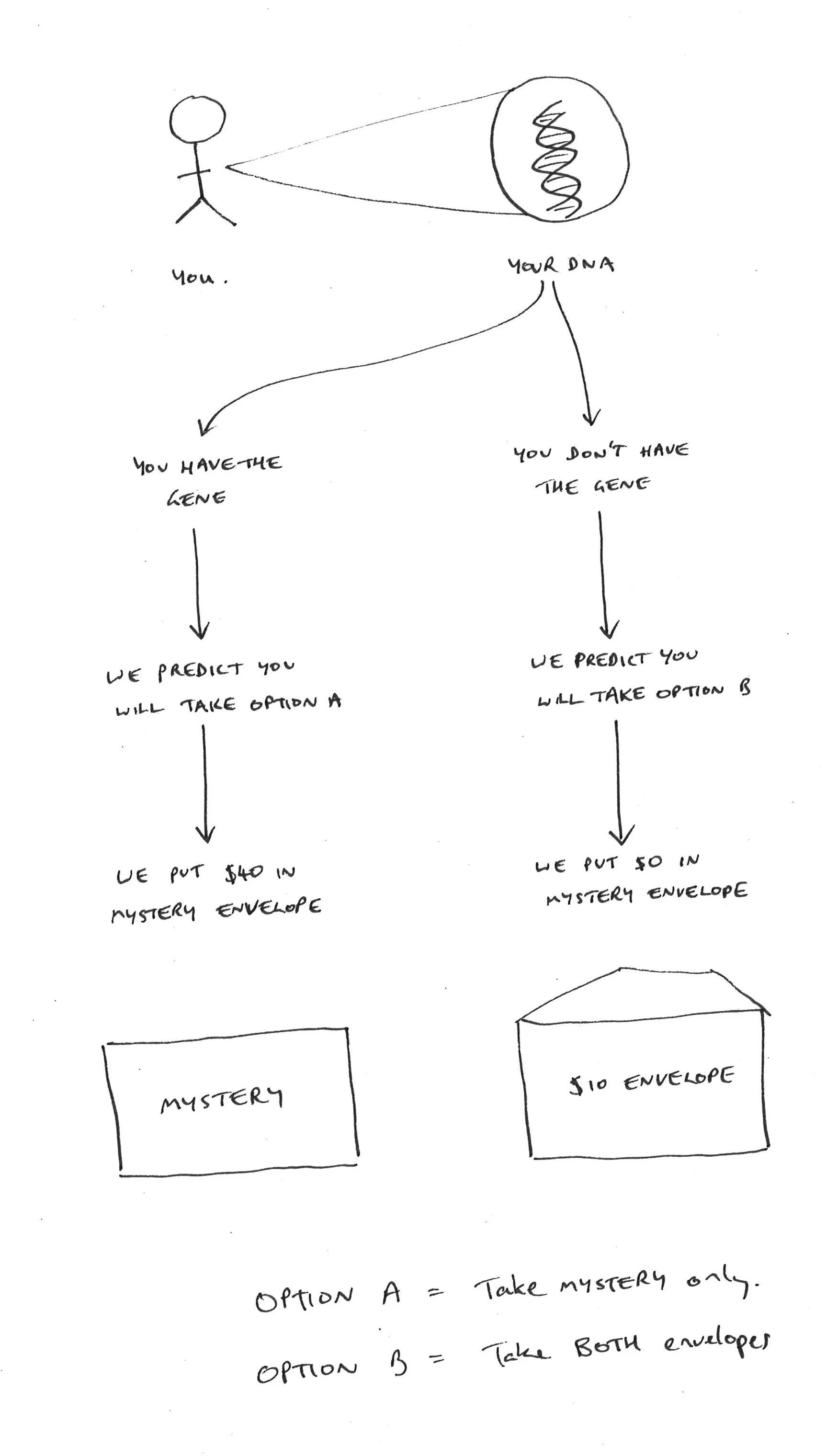
Now what’s rational? The orthodoxy is you should definitely take both envelopes (option B). There is a dominance argument to that effect: no matter what gene we thought you had, you are going to do better by taking both than you would do if you took option A alone. The contents of the Mystery envelope are fixed, so you may as well add the extra $10.

Now suppose you’ve been convinced by this argument (I’m not insisting you should be, I’m just interested in the epistemic position of someone in this state). Then you are leaning towards the “causal decision theory” side of the debate. The other side of the debate is the “evidential decision theory” side, which would recommend taking option A.

Having been convinced of this argument to adopt a CDT-friendly position, suppose I told you that, “when I tweak the amounts of money involved, the probabilities, and so on, some people change their minds, and prefer option A”. Should this undermine your confidence in your judgment that you should definitely take option B?

It might undermine your confidence a bit if you have a limited imagination, and can’t quite work out how changing the amounts might change things. But consider how it might be different.

The confidence of the prediction might be higher or lower. Let’s stipulate that the genetic prediction is always at least .5 accurate. But if it became more accurate – say 0.75 or 0.9 – would that make you waver in your intention to take the second envelope?
The amount that we have placed in the second envelope might be greater. But the greater it is, then prima facie there is even more reason to take both envelopes. On the other hand, it might be lesser. If it were very small, maybe it would become so small that the dominance argument would not be very appealing any more. But let’s just focus on cases where the amount in the second envelope increases. This seems unlikely to change your preference for Option B.
The amount that might be placed in the Mystery envelope might be greater. But of course, it doesn’t matter how much it might be, you still know that by taking both envelopes you get all the money you can possibly get.[2]

So if you accept the dominance argument, changing the amounts in the envelopes or the probability of correct prediction changes nothing. You should still take option B.

Now suppose you discover that the original thought experiment involved amounts of money, and degrees of probability, that are relatively extreme. The amount that might be placed in the Mystery envelope is $1 million. The amount that is already placed in the second envelope is $1000. And the probability that we have correctly predicted your choice is 0.999 or somesuch. And further, you learn that almost everyone presented with this scenario chooses option A. Is this any reason to give up your initial verdict, that B is the correct option, regardless of the amounts and the probabilities? (This is essentially the original Newcomb case, for those not already familiar.)

Together with collaborators Adam Bales and Josh May, I’ve been working on the design of an experiment that explores intuitions about Newcomb’s case from this sort of angle. Our hunch is that the extreme parameters used in Newcomb’s original case are bad news for the reliability of the intuitions it generates. That’s not to say that causal decision theory is definitely correct – just that it is strange/risky/ill-advised to rely on intuitions about such an extreme scenario to inform our beliefs about the nature of rational choice, when it seems very unlikely that people would have similar beliefs about more mundane versions of that scenario.

The design, rough idea

Our hypothesis is: subjects show stake sensitivity (sensitivity to the amounts of money and the probabilities) in extreme versions of Newcomb cases that is different from the stake sensitivity they show in mundane versions. Roughly, a causal decision theorist should be insensitive to the stakes, whereas an evidential decision theorist says you should regard the gamble I presented at the beginning (without any complicated genetic story) as identical to the Newcomb case: in both scenarios you should be sensitive to how much money is on offer, in a way that depends on your risk aversion and utility function for money.

In particular, we hypothesise that subjects will show low stake sensitivity in Newcomb cases where the probabilities and amounts are moderate, and high stake sensitivity where the probabilities and amounts are extreme. In order to get a handle on what high or low stake sensitivity is, we propose to run treatments in which subjects are asked about Newcomb cases and also treatments in which subjects are asked about non-Newcomb, parallel, “Vanilla” gambles – just like the choice I first presented above. These gambles are parallel in the sense that an evidential decision theorist regards them as identical, but because they don’t involve any of the funny backstory that is essential to Newcomb cases, the two types of decision theory agree about what is rational. So that gives us four broad treatment categories in a 2 by 2 design: Newcomb versus “Vanilla”; and Extreme parameters (e.g. 0.999 probabilities, hundreds of thousands of dollars at stake) versus Mundane parameters (e.g. 2/3 probabilities, tens of dollars at stake). Within those four treatment groups, we need one further binary condition that changes one of the stakes factors – say the amount that goes in the Mystery envelope. In “high” treatments this amount will be greater, making it ostensibly more tempting to go for option A – at least in the Vanilla cases.

The parameters of the various treatments are summarised below, omitting the Newcomb/Vanilla variable.

Extreme/Mundane	High/Low	Option A	Option B
Mundane	Low	(2/3, $30; 1/3, $0)	(2/3, $10; 1/3, $40)
Mundane	High	(2/3, $50; 1/3, $0)	(2/3, $10; 1/3, $60)
Extreme	Low	(0.99, $200,000; 0.01, $0)	(0.99, $1,000; 0.01, $201,000)
Extreme	High	(0.99, $1,000,000; 0.01, $0)	(0.99, $1,000; 0.01, $1,001,000)

So we can make the following comparisons:

Mundane-Vanilla-High versus Mundane-Vanilla-Low gives us a measure of how much is normal stakes sensitivity when the parameters are mundane.
Then we compare how people behave in Mundane-Newcomb-High versus Mundane-Newcomb-Low.

We predict that there will be a big difference: very few people will show similar stakes sensitivity in the Newcomb variant.

Then we can make the same sort of comparison for the extreme parameters:

Extreme-Vanilla-Low vs Extreme-Vanilla-High gives us a baseline of how much difference it makes to offer, say $1 million versus $200,000 in envelope A, before taking into account the strangeness of a Newcomb puzzle.
Then we compare the Extreme-Newcomb cases to see how much stakes sensitivity is displayed between Low and High.

We predict that there will be much less of a difference. When the parameters are extreme, people will tend to be stakes sensitive in Newcomb cases, where they are not stakes sensitive when the parameters are moderate.

Suppose we’ve got that bit right. The question is: can we draw the sort of inference we hope to from this sequence of comparisons? (I’m going out on a limb here, perhaps beyond what my co-authors would like.) I’m inclined to say that a pattern of results like that reinforces that Newcomb’s original puzzle may be a very doubtful thought experiment. It is relying on extreme parameters, well beyond the normal range of human decision making experience, and so if it elicits an anomalous response, we should be wary of trusting that response as reliable or justified.

Is that fair? If you can, please shoot this idea down, before we spend money on doing the experiment. :)

For a taste of some of the work done by economists on trying to measure risk aversion accurately, using real stakes, this is a seminal paper: Holt, C. A., & Laury, S. K. (2002). Risk aversion and incentive effects. American Economic Review. ↩
Of course, there’s more that might be said here, for someone who is a convinced one-boxer (EDT theorist), but I’m trying to keep this short, and focus on how a CDT-inclined person should change their opinion, if at all, under changes in stakes. ↩